Your Diagram showing law of demand images are available in this site. Diagram showing law of demand are a topic that is being searched for and liked by netizens now. You can Download the Diagram showing law of demand files here. Download all royalty-free images.
If you’re looking for diagram showing law of demand images information linked to the diagram showing law of demand keyword, you have come to the right blog. Our site always gives you hints for seeing the maximum quality video and image content, please kindly surf and find more informative video content and images that fit your interests.
Diagram Showing Law Of Demand. However economic growth means demand continues to rise. The effect is to cause a large rise in price. The relationship between quantity and price will follow the demand curve as long as the four determinants of demand dont change. Conversely as the rates of a product decrease the quantity demanded increases.
 Diagrams Showing How Shifts In The Demand And Supply Curves Changes The Market Equilibrium Equilibrium Supply Economics From pinterest.com
Log Q P log 3 2 log P displaystyle log Q Plog 3-2log P Note that really a demand curve should be drawn with price on the horizontal x -axis since it is the independent variable. The law of demand states that an increase in price leads to a decrease in demand. The market for newspapers in your town. But just following on of what I just said following the law of demand at a low price this is associated with if we go to the demand curve a high quantity demanded quantity demanded two. Thus there exists an inverse relationship between price and quantity demanded of a commodity. In the figure point P of the demand curve DD 1 shows demand for 100 units at the Rs.
This relationship follows the law of demand which states that the quantity demanded will drop as the price rises all other things being equal.
Other things remaining constant. The law of demand states that other things remaining constant the quantity demanded of a commodity decreases with rise in its price and increase with a fall in its price. Log Q P log 3 2 log P displaystyle log Q Plog 3-2log P Note that really a demand curve should be drawn with price on the horizontal x -axis since it is the independent variable. Conversely as the rates of a product decrease the quantity demanded increases. Understanding law of demand using demand schedule. Demand Schedule is a tabular representation of various combinations of price and quantity demanded by a consumer during a particular period of time.
 Source: pinterest.com
This is explained with the help of a table and Figure Both demand schedule and following demand. This relationship follows the law of demand which states that the quantity demanded will drop as the price rises all other things being equal. Understanding law of demand using demand schedule. The Law of Demand. So there is an inverse relationship between price and quantity demanded of a commodity.
 Source: pinterest.com
The quantity demanded is an amount per unit of time. Law of demand- This law states that other things remain constant a consumer purchases more quantity of a commodity at lesser price and less quantity at higher pricesIt means there is inverse relationship between price of commodity and quantity demanded. The functional relationship between price and quantity demanded can be represented as Dx f. An increase in demand leads to higher price and higher quantity. For example the amount per day or per month.
 Source: in.pinterest.com
The Law of Demand states that when the price of a commodity falls its demand increases and when the price of a commodity rises its demand decreases. Instead price is put on the vertical f x y -axis as a matter of unfortunate historical convention. Demand curve is a graphic representation of the demand schedule. An imaginary demand schedule is given below. Thus there exists an inverse relationship between price and quantity demanded of a commodity.
 Source: pinterest.com
Demand Curve or Diagram. The Law of Demand. B DP constant which represents the change in Dx produced by Px On the other hand in the long run demand function shows a relationship between the aggregate demand of a product and a number of determinants of demand such as price consumers income standard of living and price of substitutes. Thus there exists an inverse relationship between price and quantity demanded of a commodity. It can be expressed as D f P that is demand is a function of price.
 Source: pinterest.com
The number of buyers can also affect demand. Log Q P log 3 2 log P displaystyle log Q Plog 3-2log P Note that really a demand curve should be drawn with price on the horizontal x -axis since it is the independent variable. As the price falls to the new equilibrium level the quantity supplied decreases to 20 million pounds of coffee per month. The downward-sloping marginal utility curve is transformed into the downward-sloping demand curve. The Law of Demand.
Source: pinterest.com
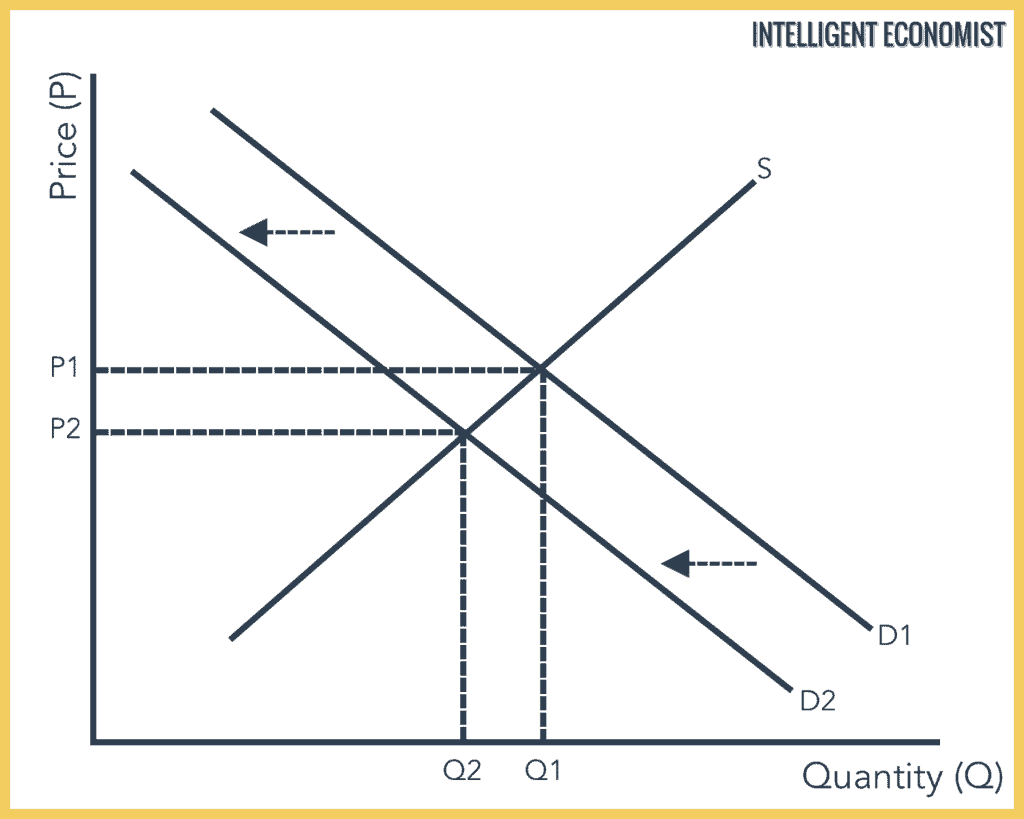
5 where price is also measured on the Y-axis marginal utility curve MU becomes the demand curve. This is explained with the help of a table and Figure Both demand schedule and following demand. From the diagram when the price is at P1 the quantity demanded is Q1 and when the prices move to P2 the quantity demanded reduces to Q2. The quantity demanded is an amount per unit of time. The salaries of journalists go up.
 Source: pinterest.com
The relationship between quantity and price will follow the demand curve as long as the four determinants of demand dont change. It can be expressed as D f P that is demand is a function of price. As the preceding situation demonstrates the law of demand establishes. The number of buyers can also affect demand. These points are then graphed and the line connecting them is the demand curve.
 Source: pinterest.com
Creately diagrams can be exported and added to Word PPT powerpoint Excel Visio or any other document. The factors that influence the demand for a commodity are known as determinants of demand. This is the famous Marshallian Law of Demand. Other things remaining constant. Aside from price factors that affect demand are consumer income preferences expectations and prices of related commodities.
 Source: pinterest.com
And so to be very particular about this quantity demanded is associated with a particular point on the demand curve while the demand curve is the set of. Instead price is put on the vertical f x y -axis as a matter of unfortunate historical convention. An increase in demand leads to higher price and higher quantity. Aside from price factors that affect demand are consumer income preferences expectations and prices of related commodities. Other things remaining constant.
 Source: pinterest.com
Understanding law of demand using demand schedule. Demand Schedule is a tabular representation of various combinations of price and quantity demanded by a consumer during a particular period of time. The salaries of journalists go up. B DP constant which represents the change in Dx produced by Px On the other hand in the long run demand function shows a relationship between the aggregate demand of a product and a number of determinants of demand such as price consumers income standard of living and price of substitutes. The Law of Demand states that when the price of a commodity falls its demand increases and when the price of a commodity rises its demand decreases.
 Source: pinterest.com
For example the amount per day or per month. The equilibrium price falls to 5 per pound. So there is an inverse relationship between price and quantity demanded of a commodity. The Law of Demand. The Law of Demand states that when the price of a commodity falls its demand increases and when the price of a commodity rises its demand decreases.
 Source: pinterest.com
The downward-sloping marginal utility curve is transformed into the downward-sloping demand curve. The Law of Demand. Demand can be visually represented by a demand curve within a graph called the demand schedule. Diagram showing Increase in Price. This law can be explained with the help of demand schedule and demand curve as presented below.
 Source: pinterest.com
Instead price is put on the vertical f x y -axis as a matter of unfortunate historical convention. Creately diagrams can be exported and added to Word PPT powerpoint Excel Visio or any other document. Panel b of Figure 310 Changes in Demand and Supply shows that a decrease in demand shifts the demand curve to the left. So there is an inverse relationship between price and quantity demanded of a commodity. An imaginary demand schedule is given below.
 Source: pinterest.com
In this diagram we have rising demand D1 to D2 but also a fall in supply. As the price falls to the new equilibrium level the quantity supplied decreases to 20 million pounds of coffee per month. The functional relationship between price and quantity demanded can be represented as Dx f. Thus there exists an inverse relationship between price and quantity demanded of a commodity. The law of demand states that other things remaining constant the quantity demanded of a commodity decreases with rise in its price and increase with a fall in its price.
 Source: pinterest.com
The equilibrium price falls to 5 per pound. The Law of Demand. The demand schedule shows that as price rises quantity demanded decreases and vice versa. Understanding law of demand using demand schedule. Demand curve which shows the relation between price of a commodity and quantity demanded of that commodity that consumer wishes to purchase is called demand curve.
 Source: pinterest.com
The law of demand states that an increase in price leads to a decrease in demand. So there is an inverse relationship between price and quantity demanded of a commodity. Creately diagrams can be exported and added to Word PPT powerpoint Excel Visio or any other document. This is explained with the help of a table and Figure Both demand schedule and following demand. In the figure point P of the demand curve DD 1 shows demand for 100 units at the Rs.
 Source: pinterest.com
The law of demand can be seen in US. Similarly the law of demand in economics is an interesting chapter that also includes some related sub-topics like exceptions of this law and so on. The functional relationship between price and quantity demanded can be represented as Dx f. This indicates the inverse relation between price and. Aside from price factors that affect demand are consumer income preferences expectations and prices of related commodities.
 Source: pinterest.com
From the diagram when the price is at P1 the quantity demanded is Q1 and when the prices move to P2 the quantity demanded reduces to Q2. Show in a diagram the effect on the demand curve the supply curve the equilibrium price and the equilibrium quantity of each of the following events. Instead price is put on the vertical f x y -axis as a matter of unfortunate historical convention. Demand curve is a graphic representation of the demand schedule. The quantity demanded is an amount per unit of time.
This site is an open community for users to share their favorite wallpapers on the internet, all images or pictures in this website are for personal wallpaper use only, it is stricly prohibited to use this wallpaper for commercial purposes, if you are the author and find this image is shared without your permission, please kindly raise a DMCA report to Us.
If you find this site convienient, please support us by sharing this posts to your own social media accounts like Facebook, Instagram and so on or you can also save this blog page with the title diagram showing law of demand by using Ctrl + D for devices a laptop with a Windows operating system or Command + D for laptops with an Apple operating system. If you use a smartphone, you can also use the drawer menu of the browser you are using. Whether it’s a Windows, Mac, iOS or Android operating system, you will still be able to bookmark this website.